Carrot and Stick - Part 4 - Double DQN

01 Apr 2020 in Machine Learning

One Line Fix for a Systematic Bias

In the previous post we built Deep Q Learning and saw it converge to near-perfect performance on CartPole. DQN works, but it has a known flaw baked into its update rule — one that causes it to systematically overestimate Q-values, and one that requires a single line of code to fix. That fix is Double DQN.

The Problem: Overestimation

Recall the DQN target: $$y_t = r_t + \gamma \max_{a'} Q(s_{t+1}, a';\, \theta^{-})$$

The target network picks the action with the highest Q-value in the next state and uses that value as the training target. This involves two operations in one step: selecting which action is best, and evaluating how good it is — both performed by the same network.

The problem comes from what the max operation does to noise. The network’s estimates are noisy — each one is roughly the true value plus some error that varies from update to update. For any individual action, that noise cancels out over time: sometimes the estimate is too high, sometimes too low, on average it converges. But DQN does not look at actions individually. It takes the max over all of them, and the max always picks whichever action happened to get the most positive noise this time. An underestimated action never wins; by definition, only the most overestimated one does.

A simple example makes this concrete. Suppose two actions both have a true value of 1.0. On one update the network produces [0.7, 1.4]: the max picks 1.4. On another it produces [1.3, 0.8]: the max picks 1.3. The individual noise cancels out — the average of [0.7, 1.3] is 1.0, and of [1.4, 0.8] is 1.1 — but the max does not cancel. It always returns the larger of two noisy numbers, so its expected value stays above 1.0 no matter how many updates run.

This is a mathematical certainty, not a quirk of the training setup: the expected maximum of noisy estimates is always at least as large as the true maximum, and usually larger. More actions and more noise make it worse. We then use that inflated value as the training target, which pushes the network to produce even higher estimates, which inflates the max further. The bias compounds with every gradient step.

We can measure this directly. The chart below tracks two quantities throughout training: the Q-value the network assigns to a fixed set of states (solid line), and the actual discounted return earned from those same states under the current greedy policy (dotted line). Accurate estimates would make the two lines overlap; the gap between them is the overestimation bias.

DQN’s estimated Q-values (solid red) climb well above the true returns (dotted red) as training progresses. The fix — shown in blue — is discussed next.

The Fix: Decouple Selection from Evaluation

The root cause is circular: the target network selected $a_2$ precisely because its own estimate of $a_2$ was highest, and then it used that same optimistic estimate as the training target. The selection and the evaluation are two expressions of the same error.

The fix, introduced by van Hasselt et al. in 2015, is to split these two responsibilities across the two networks we already have.

DQN — the target network both selects and evaluates: $$y_t = r_t + \gamma \, Q\!\left(s_{t+1},\; \underset{a'}{\arg\max}\; Q(s_{t+1}, a';\, \theta^{-});\; \theta^{-}\right)$$

Double DQN — the main network selects, the target network evaluates: $$y_t = r_t + \gamma \, Q\!\left(s_{t+1},\; \underset{a'}{\arg\max}\; Q(s_{t+1}, a';\, \theta);\; \theta^{-}\right)$$

Before explaining why this helps, it is worth being precise about how the two networks are actually maintained.

Only the main network $\theta$ is trained by gradient descent — its weights are updated on every training batch. The target network $\theta^{-}$ is never trained directly. Instead, every $N$ steps, its weights are simply overwritten with a copy of the main network’s current weights: $\theta^{-} \leftarrow \theta$. Between those refreshes, it stays frozen.

So the target network is not a separate learner — it is a snapshot of the main network from $N$ steps ago. The two networks differ because the main network has received many gradient updates since the last copy, while the target network has not moved at all.

Why does this help? When the main network picks $a_2$, it does so because its most recent gradient updates pushed its estimate of $a_2$ high. The target network reflects an older version of those weights — before those updates happened. It has not yet been shaped by the same recent experience, so it has no particular reason to rate $a_2$ as highly. Its estimate of $a_2$ is whatever the main network thought $N$ steps ago, which is less likely to share the same current overestimation.

In concrete terms: the main network picks $a_2$ with an estimate of 1.8 (true value 1.0). The target network, queried for that same action, gives 1.3 — not because it is wiser, but because it did not select $a_2$ and therefore carries no inflated expectation for it. The training target becomes $r + \gamma \cdot 1.3$ instead of $r + \gamma \cdot 2.1$, and over many updates the Q-values stop drifting upward.

The diagram below shows the two paths side by side:

Implementation

The change is exactly one line in the training step.

DQN target computation:

target = reward + gamma * target_network(next_state).max(dim=1)[0] * (1 - done)

Double DQN target computation:

best_actions = main_network(next_state).argmax(dim=1)
target = reward + gamma * target_network(next_state).gather(1, best_actions.unsqueeze(1)).squeeze() * (1 - done)

Instead of taking the max directly from the target network, we first ask the main network which action it thinks is best, then ask the target network what that action is actually worth. Everything else — the replay buffer, the target network refresh, the loss function, the game loop — stays identical.

Results

CartPole: the bias hides

On CartPole, both algorithms reach the ceiling quickly and finish in the same place.

This is not evidence that the bias does not exist — the overestimation chart from earlier shows it clearly. It is evidence that CartPole is too short and too simple for the bias to matter. Episodes end in at most 200 steps, the state space has four variables, and there are only two actions. The inflated Q-values never accumulate long enough to push training in the wrong direction.

LunarLander: the bias compounds

LunarLander is a harder test. The lander has eight state variables, four discrete actions, and has to learn to fire its main and side thrusters in a precise sequence to touch down between two flags without crashing. The reward is shaped but delayed — hovering costs fuel, crashing deducts 100, a clean landing adds up to 140. That combination of longer episodes, delayed payoffs, and a richer action space is exactly where overestimation compounds. Each inflated target raises the Q-values of nearby states, which inflates the next set of targets, and the spiral has hundreds of steps to build.

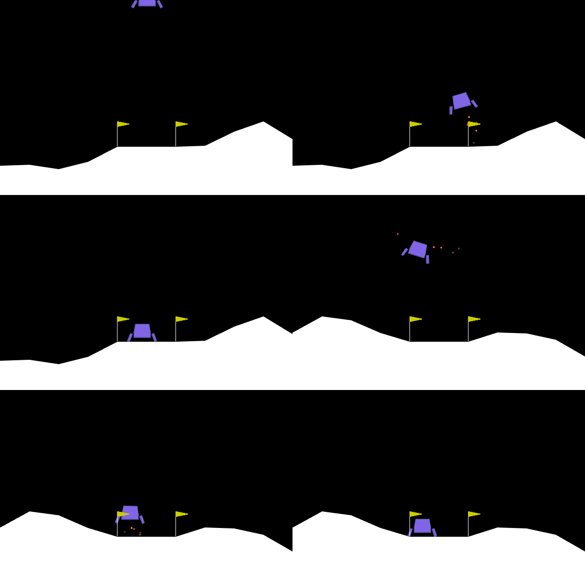
Both algorithms eventually converge on most seeds, which already tells you something: the bias does not prevent learning, it just makes it harder. Where the difference shows up is in the early and middle phases. DQN’s estimated Q-values — as the overestimation chart showed — climb well above the true returns. That inflation does not cause a catastrophic failure on LunarLander, but it does make the learning noisier: the targets the network is trained against are moving targets that drift upward, and the agent has to learn through that drift rather than against stable ground truth. Double DQN removes the drift. The targets are still noisy, but they are not systematically inflated, and the network converges toward something that more closely matches what the actions are actually worth. The final reward difference between the two is modest — the bias does not need to change who wins to matter, it just makes the path to convergence noisier and less predictable, which is what the overestimation chart earlier in this post already showed directly.

Conclusion and Next Steps

Double DQN is a minimal change — one line — that removes a systematic source of instability. On a toy environment like CartPole you would never know it was there. On anything with delayed rewards and a meaningful action space, it is the difference between an algorithm that converges reliably and one that depends on luck.

The next extension in this direction is Dueling DQN, which changes the network architecture itself. Instead of outputting Q-values directly, the network learns two separate quantities: how good it is to be in a state at all (the value), and how much better each action is relative to the average (the advantage). The Q-value is their sum. This decomposition makes learning more efficient, especially in states where the choice of action barely matters — the network can update its estimate of the state’s value from every transition, not just the ones where a specific action was taken.