Not All Who Wander Are Lost

01 Mar 2019 in Machine Learning

A Quick Start Guide to Multi Armed Bandits

Decisions are hard, they have always been. And when you finally find something you like, there is always that thought, in the back of your head - “can I find something better?”.

One of the challenges that arise in Reinforcement Learning is the Exploration - Exploitation Dilemma, do we choose - exploitation, where we make the best decision given current knowledge or exploration, where we gather more knowledge that might lead us to better decisions in the future.

In this post we will introduce the Multi Armed Bandits (MAB) problem, show two algorithms that solve this problem, and run a simulation.

Multi Armed Bandits

The MAB problem, or bandit problem for short, is one of the simplest instances of the sequential decision making problem, in which a learner needs to select options from a given set of alternatives repeatedly in an online manner. The name comes from the gambling world in which a gambler decides from a row of slot machines, sometimes known as “one-armed bandits”.

Algorithms

Before we get to the good stuff we need to understand what we are trying to achieve. As described, the MAB problem is a sequential decision making problem.

The “game” is set like this: in each round the agent decides on an action or arm x from a finite set X, pulls the arm and receives a reward.

Each arm’s reward is associated with a probability distribution over [0, 1], each with an expectation μ. We will assume the existence of a unique best arm: $$x^* = \operatorname{argmax}_{x \in X}(\mu_x)$$

To sum things up:

Symbol	Meaning
x ∈ X	The arms
μ_x	Mean reward of arm x
u_t	Reward received at round t

The object of the game is to minimize the cumulative regret, defined as: $$R(T) = \sum_{t=1}^{T} \mu_{x^*} - u_t$$

The cumulative regret shows the difference between the reward the player could have acquired if they always played the best arm and the sum of rewards actually acquired.

Lets start with the naive case - assuming we have K arms and T rounds to play, and we decide to play each arm T/K times - the regret we would endure is linear with T. But we can do better!

UCB

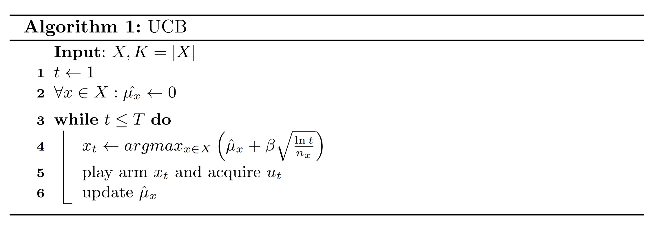
The most commonly used algorithm for the MAB setting, the UCB algorithm minimizes cumulative regret by picking the arm with the highest Upper Confidence Bound in each round: $$x_t = \operatorname{argmax}_{x \in X} \left( \hat{\mu}_x + \beta\sqrt{\frac{\ln t}{n_x}} \right)$$

The left term is the empirical mean reward of the arm; the right term is the exploration bonus, which shrinks as the arm is pulled more. At each round, the chosen arm is the one that potentially has the highest reward — either because it has not been tried enough, or because its average reward has been promising. β acts as a regulator and can be set to 1.

The UCB algorithm guarantees logarithmic regret in T and is implemented as follows:

class UCB:
    def __init__(self, n_arms, beta=1.0):
        self.counts = np.zeros(n_arms)   # n_x: pulls per arm
        self.mu_hat = np.zeros(n_arms)   # empirical mean per arm
        self.beta = beta

    def select_arm(self, t):
        for arm in range(len(self.counts)):
            if self.counts[arm] == 0:    # pull each arm at least once
                return arm
        ucb = self.mu_hat + self.beta * np.sqrt(np.log(t) / self.counts)
        return int(np.argmax(ucb))

    def update(self, arm, reward):
        self.counts[arm] += 1
        n = self.counts[arm]
        self.mu_hat[arm] = ((n - 1) * self.mu_hat[arm] + reward) / n

Thompson Sampling

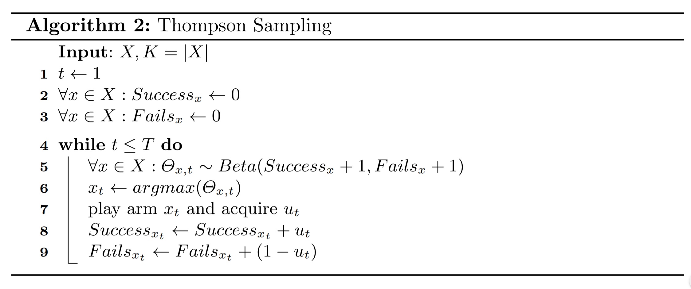
The basic idea is to choose an arm according to its probability of being the best arm. The algorithm maintains success and failure counts for each arm and holds a Beta-distributed random variable for each: $$\Theta_x \sim \text{Beta}(\text{Success}_x + 1,\ \text{Failures}_x + 1)$$

At each round, all random variables are sampled and the arm with the highest sample is chosen: $$x_t = \operatorname{argmax}_{x \in X}\ \Theta_{x,t}$$

The Thompson Sampling algorithm also guarantees logarithmic regret in T and is implemented as follows:

class ThompsonSampling:
    def __init__(self, n_arms):
        self.successes = np.ones(n_arms)
        self.failures  = np.ones(n_arms)

    def select_arm(self):
        samples = np.random.beta(self.successes, self.failures)
        return int(np.argmax(samples))

    def update(self, arm, reward):
        self.successes[arm] += reward
        self.failures[arm]  += 1 - reward

Implementation

In order to simulate a game we need to implement the arms. We will use a Bernoulli arm, which draws a reward of 0 or 1 according to its mean:

class BernoulliArm:
    def __init__(self, p):
        self.p = p

    def draw(self):
        return 1 if np.random.random() < self.p else 0

Simulation

To compare the algorithms we run a simulation with 5 arms (mean rewards drawn randomly), 1000 rounds per run, and 500 runs. The chart shows mean cumulative regret with ± one standard deviation:

Thompson Sampling accumulates less regret and converges faster. UCB is more conservative in its exploration — it requires hard evidence before committing to an arm, while Thompson Sampling reasons probabilistically from the start.

Conclusion

In this post we have defined the Multi Armed Bandit problem, showed two solutions and compared between them using a simulation.

In the next post we will show several other solutions that can handle different environments, such as partial information about the reward.